In the world of machine learning, it's not just about making predictions, but about being sure of those predictions. Think about an autonomous car that needs to make a decision on whether to stop at an intersection or not, or a healthcare AI diagnosing a patient's condition-the confident scores will tell how sure a model can be about its predictions, as it will aid businesses and decision-makers to then act with greater assurance.

However, like humans, machine learning models sometimes make mistakes when predicting a value from an input data point. But also like humans, most models are able to provide information about the reliability of these predictions. When you say  “I’m sure that…” or “Maybe it is…”, you are actually assigning a relative qualification to how confident you are about what you are saying. In mathematics, this information can be modeled, for example as a percentage, i.e. a number between 0 and 1, and most machine learning technologies provide this type of information: the confidence score.

A human-to-machine equivalence for this confidence level could be:

“I’m sure that…” <=> 100%

“I think it is…” <=> 70%

“I don’t know but I’d say…” <=> <50%

The main issue with this confidence level is that you sometimes say “I’m sure” even though you’re effectively wrong, or “I have no clue but I’d say…” even if you happen to be right. Obviously, in a human conversation, you can ask more questions and try to get a more precise qualification of the reliability of the confidence level expressed by the person in front of you. But when you’re using a machine learning model and you only get a number between 0 and 1, how should you deal with it?

Why confidence scores matter

Confidence scores are more than just abstract numbers floating around in your machine learning pipeline; they form the linchpin that could make or break your entire model's effectiveness when it comes to real-world scenarios.

Think about it: would you want a model to approve a loan, flag some transaction as suspicious, or diagnose a patient if it couldn't tell you how sure it is of its predictions? That's where confidence scores come into play!

Imagine operating an e-commerce website powered by a recommendation engine that advises your customers on what to purchase. A model with a high confidence score would be able confidently to push, for instance, some new product, knowing it's likely to convert. But if it's only 60% sure, you might hold off on that recommendation and show a more reliable best-seller product. This nuanced decision-making is not just smart; rather, it directly increases your sales while keeping your customers happy.

Confidence scores become even more critical in healthcare. Say, for example, the model is working with doctors to diagnose diseases. If a model predicts the diagnosis with 98% confidence, that is okay for the doctors; they have something for a supporting opinion. But when that falls to, say, 55%, it is time for double-checking and running further tests. For life-and-death cases, these scores are not numbers but that thin second line of assurance that may just help save lives.

Or consider a world of fraud detection in financial services: if it flags a transaction as fraudulent at 95% confidence, you can easily block that transaction, knowing you will notify the customer. If that score is around 70%, it is probably better to notify the customer but allow the transaction to proceed-minimizing unnecessary friction while protecting accounts.

In all these cases, confidence scores help you strike the right balance between automation and human intervention-between risk and reward. They're the secret sauce that makes machine learning not just smart, but also practical, reliable, and safe!

Most common machine learning confidence scores

There is no standard definition of the term “confidence score” and you can find many different flavors of it depending on the technology you’re using. But in general, it’s an ordered set of values that you can easily compare to one another.

The three main confidence score types you are likely to encounter are:

Important technical note: You can easily jump from option #1 to option #2 or option #2 to option #1 using any bijective function transforming [0, +∞[ points in [0, 1], with a sigmoid function, for instance (widely used technique). Bear in mind that due to floating point precision, you may lose the ordering between two values by switching from 2 to 1, or 1 to 2. Try out to compute sigmoid(10000) and sigmoid(100000), both can give you 1.

Some machine learning metrics to understand the problem

Most of the time, a decision is made based on input. For example, if you are driving a car and receive the “red light” data point, you (hopefully) are going to stop.

When you use an ML model to make a prediction that leads to a decision, you must make the algorithm react in a way that will lead to a less dangerous decision if it’s wrong, since predictions are by definition never 100% correct.

To better understand this, let’s dive into the three main metrics used for classification problems: accuracy, recall and precision. We can extend those metrics to other problems than classification.

True positives, true negatives, false positives, and false negatives

These definitions are very helpful to compute the metrics. In general, they refer to a binary classification problem, in which a prediction is made (either “yes” or “no”) on data that holds a true value of “yes” or “no”.

In the next sections, we’ll use the abbreviations tp, tn, fp and fn.

Accuracy

Accuracy (or acc) is the easiest metric to understand. It’s simply the number of correct predictions on a dataset. Given a test dataset of 1,000 images for example, in order to compute the accuracy, you’ll just have to make a prediction for each image and then count the proportion of correct answers among the whole dataset.

Let’s say you make 970 good predictions out of those 1,000 examples: this means your algorithm accuracy is 97%.

This metric is used when there is no interesting trade-off between a false positive and a false negative prediction.

But sometimes, depending on your objective and the gravity of your decisions, you want to unbalance the way your algorithm works using other metrics such as recall and precision.

Accuracy formula: ( tp + tn ) / ( tp + tn + fp + fn )

Recall (also known as sensitivity)

To compute the recall of your algorithm, you need to consider only the real ‘true’ labelled data among your test dataset, and then compute the percentage of right predictions. It’s a helpful metric to answer the question: “On all the true positive values, which percentage does my algorithm actually predict as true?”

If an ML model must predict whether a stoplight is red or not so that you know whether you must  your car or not, do you prefer a wrong prediction that:

1. says ‘red’ although it’s not
2. says ‘not red’ although it is

Let’s figure out what will happen in those two cases:

1. Your car stops although it shouldn’t. It’s only slightly dangerous as other drivers behind may be surprised and it may lead  to a small car crash.
2. Your car doesn’t  stop at the red light. This is very dangerous as a crossing driver may not see you, create a full speed car crash and cause serious damage or injuries..

Everyone would agree that case (b) is much worse than case (a). In this scenario, we thus want our algorithm to never say the light is not red when it is: we need a maximum recall value, which can only be achieved if the algorithm always predicts “red” when the light is red, even if it’s at the expense of predicting  “red” when the light is actually green.

The recall can be measured by testing the algorithm on a test dataset. It’s a percentage that divides the number of data points the algorithm predicted “Yes” by the number of  data points that actually hold the “Yes” value.

For example, let’s say we have 1,000 images with 650 of red lights and 350 green lights. To compute the recall of our algorithm, we are going to make a prediction on our 650 red lights images. If the algorithm says “red” for 602 images out of those 650, the recall will be 602 / 650 = 92.6%. It’s not enough! 7% of the time, there is a risk of a full speed car accident. We’ll see later how to use the confidence score of our algorithm to prevent that scenario, without changing anything in the model.

Recall formula:  tp / ( tp + fn )

Precision (also called ‘positive predictive value’)

The precision of your algorithm gives you an idea of how much you can trust your algorithm when it predicts “true”. It is the proportion of predictions properly guessed as “true” vs. all the predictions guessed as “true” (some of them being actually “wrong”).

Let’s now imagine that there is another algorithm looking at a two-lane road, and answering the following question: “can I pass the car in front of me?”

Once again, let’s figure out what a wrong prediction would lead to. Wrong predictions mean that the algorithm says:

1. “You can overtake the car” although you can’t
2. “No, you can’t overtake the car” although you can

Let’s see what would happen in each of these two scenarios:

1. You increase your car speed to overtake the car in front of yours and you move to the lane on your left (going in the opposite direction). However, there might be another car coming at full speed in that opposite direction, leading to a full-speed car crash. Result: you are both badly injured.
2. You could overtake the car in front of you but you will gently stay behind the slow driver. Result: nothing happens, you just lost a few minutes.

Again, everyone would agree that (b) is a better scenario than (a). We want our algorithm to predict “you can overtake” only when it’s actually true: we need a maximum precision, never say “yes” when it’s actually “no”.

To measure an algorithm precision on a test set, we compute the percentage of real “yes” among all the “yes” predictions.

To do so, let’s say we have 1,000 images of passing situations, 400 of them represent a safe overtaking situation, 600 of them an unsafe one. We’d like to know what the percentage of true “safe” is among all the “safe” predictions our algorithm made.

Let’s say that among our “safe” predictions images:

• 382 of them are safe overtaking situations: truth = yes
• 44 of them are unsafe overtaking situations: truth = no

The formula to compute the precision is: 382/(382+44) = 89.7%.

It means: 89.7% of the time, when your algorithm says you can overtake the car, you actually can. But it also means that 10.3% of the time, your algorithm says that you can overtake the car although it’s unsafe. The precision is not good enough, we’ll see how to improve it thanks to the confidence score.

Precision formula: tp / ( tp + fp )

Metrics summary

You can estimate the three following metrics using a test dataset (the larger the better), and compute:

How to set effective confidence score thresholds

Confidence scores are central to interpreting the reliability of machine learning model predictions. These scores often fall within a specific interval (e.g., 0 to 1), reflecting the model's certainty about its predictions.Confidence scores in OCR tasks, for instance, are shaped during training and can be refined through methods like thresholding to improve the reliability of extracted text.

Let's take the example of a classification task: a confidence score of 0.8 might indicate that the model assigns an 80% likelihood to a given class. However, understanding these scores often requires considering confidence intervals to account for uncertainty and variability, especially when working with limited sample sizes.

In all the previous cases, we consider our algorithms only able to predict “yes” or “no”. But these predictions are never outputted as “yes” or “no”, it’s always an interpretation of a numeric score. Actually, the machine always predicts “yes” with a probability between 0 and 1: that’s our confidence score.

As a human being, the most natural way to interpret a prediction as a “yes” given a confidence score between 0 and 1 is to check whether the value is above 0.5 or not. This 0.5 is our threshold value, in other words, it’s the minimum confidence score above which we consider a prediction as “yes”. If it’s below, we consider the prediction as “no”.

However, as seen in our examples before, the cost of making mistakes vary depending on our use cases.

Fortunately, we can change this threshold value to make the algorithm better fit our requirements. For example, let’s imagine that we are using an algorithm that returns a confidence score between 0 and 1. Setting a threshold of 0.7 means that you’re going to reject (i.e consider the prediction as “no” in our examples) all predictions with a confidence score below 0.7 (included). Doing this, we can fine tune the different metrics.

In general:

• Increasing the threshold will lower the recall, and improve the precision
• Decreasing the threshold will do the opposite

The important thing to point out now is that the three metrics above are all related. A simple illustration is:

• threshold = 0 implies that your algorithm always says “yes”, as all confidence scores are above 0. You get the minimum precision (you’re wrong on every real “no” data) and the maximum recall (you always predict ”yes” when it’s a real “yes”)
• threshold = 1 implies that you reject all the predictions, as all confidence scores are below 1 (included). You have 100% precision (you’re never wrong saying “yes”, as you never say yes..), 0% recall (…because you never say “yes”)

Trying to set the best score threshold is nothing more than a tradeoff between precision and recall.

Obviously, setting the right confidence threshold depends on your business goals. Here’s a step-by-step approach to determine optimal thresholds:

1. Analyze your data: Start by evaluating the distribution of confidence scores across your predictions. Use visualization tools like histograms to see how confidence scores cluster.
2. Establish initial thresholds: For example, if 80% of your predictions have a confidence score above 90%, you might set an automated acceptance threshold at 90%.
3. Test and iterate: Continuously monitor how adjusting thresholds impacts false positives and false negatives. For instance, lowering your threshold to 85% might catch more issues but could increase the manual review workload.

The impact of confidence scores on overall accuracy is significant. During the training phase, models are exposed to diverse data to calibrate confidence outputs. Using techniques like bootstrap sampling can further refine the model's performance by estimating confidence intervals or testing robustness against various subsets of the data.

For example, a robust method to evaluate confidence scores involves testing predictions on unseen samples and assessing the alignment between confidence scores and actual outcomes.

The precision-recall curve (PR curve)

To choose the best value of the threshold you want to set in your application, the most common way is to plot a Precision Recall curve (PR curve).

To do so, you are going to compute the precision and the recall of your algorithm on a test dataset, for many different threshold values. Once you have all your couples (pr, re), you can plot this on a graph that looks like:

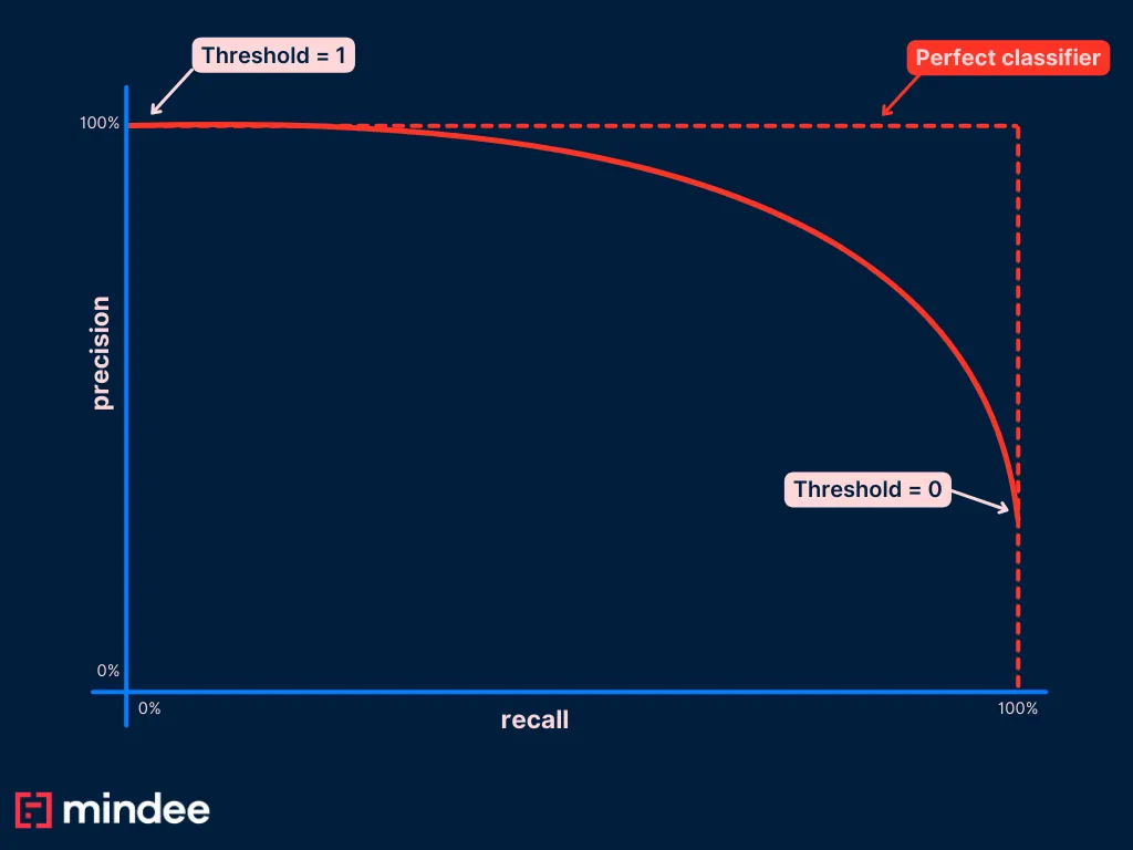
PR curves always start with a point (r=0; p=1) by convention.

Once you have this curve, you can easily see which point on the blue curve is the best for your use case. You can then find out what the threshold is for this point and set it in your application.

How to plot your PR curve?

All the previous examples were binary classification problems where our algorithms can only predict “true” or “false”. In the real world, use cases are a bit more complicated but all the previous metrics can be generalized.

Let’s take a new example: we have an ML based OCR that performs data extraction on invoices. This OCR extracts a bunch of different data (total amount, invoice number, invoice date…) along with confidence scores for each of those predictions.

Which threshold should we set for invoice date predictions?

This problem is not a binary classification problem, and to answer this question and plot our PR curve, we need to define what a true predicted value and a false predicted value are.

All the complexity here is to make the right assumptions that will allow us to fit our binary classification metrics: fp, tp, fn, tp

Here are our assumptions:

1. Every invoice in our data set contains an invoice date
2. Our OCR can either return a date or an empty prediction

If unlike #1, your test dataset contains invoices without any invoice dates present, I strongly recommend you to remove them from your dataset and finish this first guide before adding more complexity. This assumption is obviously not true in the real world, but the following framework would be much more complicated to describe and understand without this.

Now, let’s define our metrics:

• true positive: the OCR correctly extracted the invoice date
• false positive: the OCR extracted a wrong date
• true negative: this case isn’t possible as there is always a date written in our invoices
• false negative: the OCR extracted no invoice date (i.e empty prediction)

Before diving in the steps to plot our PR curve, let’s think about the differences between our model here and a binary classification problem.

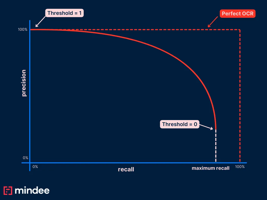
What does it mean to set a threshold of 0 in our OCR use case? It means that we are going to reject no prediction BUT unlike binary classification problems, it doesn’t mean that we are going to correctly predict all the positive values. Indeed our OCR can predict a wrong date.

It implies that we might never reach a point in our curve where the recall is 1. This point is generally reached when setting the threshold to 0. In our case, this threshold will give us the proportion of correct predictions among our whole dataset (remember there is no invoice without invoice date).

We expect then to have this kind of curve in the end:

We’re now ready to plot our PR curve.

Step 1: run the OCR on each invoice of your test dataset and store the three following data points for each

• Was the prediction correct?
• What was the confidence score for the prediction?
• Was the prediction filled with a date (as opposed to “empty”)?

The output of this first step can be a simple .csv file like this:

Step 2: compute recall and precision for threshold = 0

We need now to compute the precision and recall for threshold = 0.

That’s the easiest part. We just need to qualify each of our predictions as a fp, tp, or fn as there can’t be any true negative according to our modelization.

Let’s do the math. In the example above we have:

• 8 true positives
• 5 false positives
• 3 false negatives

In our first example with a threshold of 0., we then have:

• Precision = 8 / (8+5) = 61%
• Recall = 8 / (8+3) = 72%

We have the first point of our PR curve: (r=0.72, p=0.61)

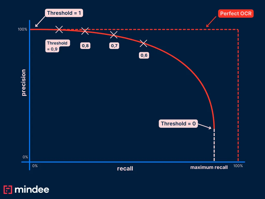
Step 3: Repeat this step for different threshold value

We just computed our first point, now let’s do this for different threshold values. We’ll take the example of a threshold value = 0.9.

As we mentioned above, setting a threshold of 0.9 means that we consider any predictions below 0.9 as empty. In other words, we need to qualify them all as false negative values (remember, there can’t be any true negative values).

To do so, you can add a column in our csv file:

In the CSV file above:

• The grey lines correspond to predictions below our threshold
• The blue cells correspond to predictions that we had to change the qualification from FP or TP to FN

Let’s do the math again.

We have:

• 6 true positives
• 3 false positives
• 7 false negatives

In our first example with a threshold of 0.9, we then have:

• Precision = 6/ (6+3) = 66%
• Recall = 6 / (6+7) = 46%

It results in a new point of our PR curve: (r=0.46, p=0.67)

Repeat this step for a set of different threshold values, and store each data point and you’re done!

Interpreting your PR curve

In a perfect world, you have a lot of data in your test set, and the ML model you’re using fits quite well the data distribution. In that case you end up with a PR curve with a nice downward shape as the recall grows, helping with the correct evaluation of your confidence score.

But a common error is that you might not have a lot of data, or you might not be using the right algorithm. In that case, the PR curve you get can be shapeless and unexploitable because of the size of your data.

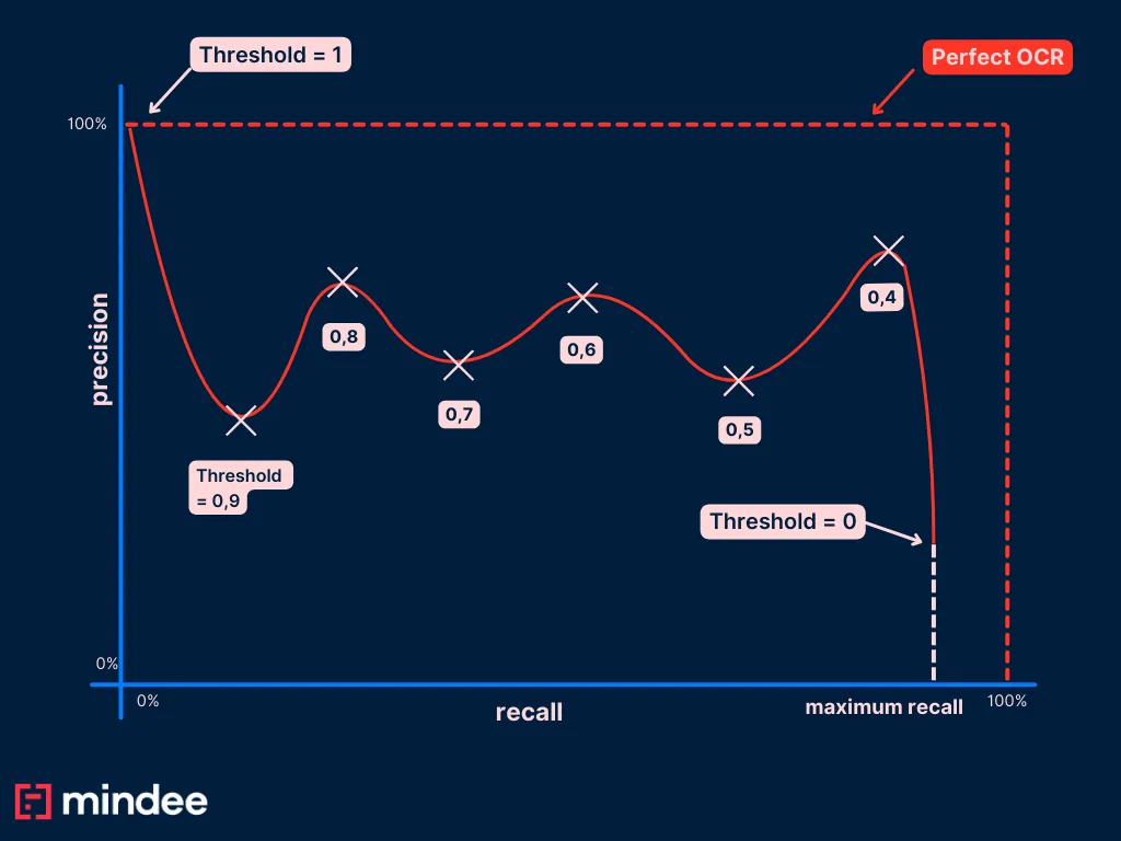
Here is an example of a real world PR curve we plotted at Mindee on a very similar use case for our receipt OCR on the date field.

We have 10k annotated data in our test set, from approximately 20 countries. The PR curve of the date field looks like this:

Confidence scores are a powerful tool to fine-tune your machine learning models and ensure they deliver accurate, actionable insights. By carefully setting thresholds and continuously monitoring performance, you can maximize the value of your models in production.

Ready to take your ML models to the next level? Check out Mindee’s powerful document processing API that leverages confidence scores to optimize data extraction. Or, dive into our blog for more tips on enhancing your machine learning workflows!